


Billboard top 100, circa 2000
Introduction
The billboard top 100 provides weekly rankings of tracks (aka singles) based on the amount of radio play, online streaming, and physical and digital sales. The number of weeks a track spends in the top 100 could be interpreted as a proxy for its popularity.
As part of my General Assembly Data Science Immersive class, I was provided a data set of tracks that made it to the top 100 around the year 2000. Given that the tracks are from circa 2000, one can assume that radio play and physical sales contributed predominantly to the rankings.
Objective
There were 2 main categories of questions that I wanted to answer:
-
Who/what took the top spot?
-
Is there anything that correlates with number of weeks spent in the top 100?
Methodology
Here’s the rough order of steps I followed in arriving at answers to these questions:
-
Get the data set into Python, and take a first look at what’s contained in the data
-
Clean the data: Rename columns as needed, deal with missing/incorrect values, change data types to make it amenable for visualization and analysis, etc
-
Plot the cleaned data to understand trends
-
Formulate a problem statement for any statistical tests that may be of interest after looking at the plots
-
Run statistical tests to draw conclusions
Dataset
The dataset contains 317 tracks by various artists/groups, with some artists/groups having multiple tracks. The track length, genre, date of entry, date of peak ranking, and weekly ranks for the 76 weeks since entry, are also included for each track. Rock seems to be predominant genre in this dataset. I added columns for number of weeks each track spent in top 100 during the 76 weeks, in addition to others to aid in analysis. Here’s a snippet of the code I used to add this column:
# Find out the number of weeks each track has been on the billboard, and average rating for each track
col_list = bb_100.columns
col_list = col_list[7:-2]
data_weeks = bb_100[col_list]

# Add these quantities to the dataframe
bb_100["num_of_weeks"] = data_weeks.count(axis=1)
bb_100["av_ranking"] = data_weeks.mean(axis=1)
Results
Who/what took the top spot?
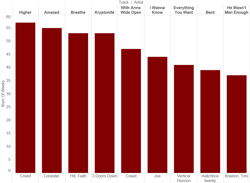
Higher, by Creed, spent the most time in the top 100 at 57 weeks, followed by Amazed (by Lonestar), Breathe (Faith Hill), Kryptonite (by 3 Doors Down) and Wide Open (by Creed again).
Creed also took the top spot in total number of weeks spent in the top 100. His tracks spent a total of 104 weeks. The next highest was Lonestar at 95 weeks, followed by Destiny’s Child at 91 weeks.
Correlation with number of weeks
1) There was no correlation between the length of a track and the time it spent in the top 100
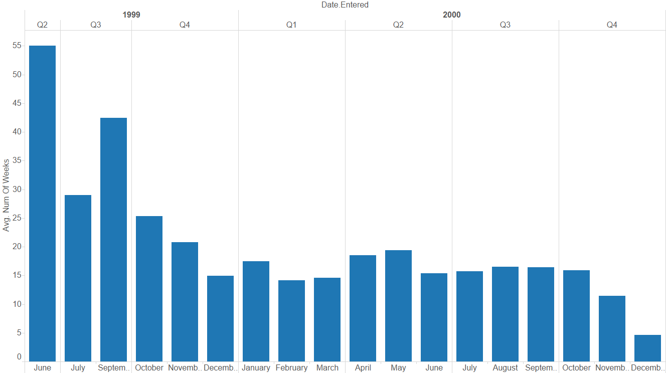
2) While it looked like tracks that entered the top 100 in Q2 and Q3 of 1999 seem to have stayed longer in the top 100, very few tracks entered the billboard during that period (<5 out of 317 total). We could explore this further if more samples from that time period were available
3) The average time spent in the top 100 seems to be genre dependent, but most genres did not have enough tracks (samples). It may be interesting to explore whether average number of weeks for Rock is significantly different than Country or Rap, all of which had enough samples to make statistical testing and drawing conclusions possible.

Statistical tests
Given the genre dependent trends observed above, I decided to run some t-tests on the number of weeks spent by Rock, Country and Rap tracks. None of these variables were normally distributed, but I assumed that their means would be normally distributed by the Central Limit Theorem, given that the number of samples (tracks) for each of these categories exceeds the recommended 30-40. The variances of all these variables were fairly different, so I used Welch’s t-tests for each pairwise comparison instead of Student t-tests.
Here’s the code I used to run the Welch’s t-test:
# Create arrays with number of weeks data for each genre of interest
rock = bb_100[bb_100["genre"] == "Rock"]["num_of_weeks"]
country = bb_100[bb_100["genre"] == "Country"]["num_of_weeks"]
rap = bb_100[bb_100["genre"] == "Rap"]["num_of_weeks"]

# Run Welch's t-test
t_rock_country = stats.ttest_ind(rock, country, equal_var=False, nan_policy='omit')
t_rock_rap = stats.ttest_ind(rock, rap, equal_var=False, nan_policy='omit')
t_country_rap = stats.ttest_ind(country, rap, equal_var=False, nan_policy='omit')
At a signifcance level of 0.05, the p-values for Rock vs Country (0.029) and Rock vs Rap (0.0025) were both <0.05, whereas it was 0.21 for Country vs Rap, implying that Rock tracks indeed performed better (stayed longer in top 100) than Country or Rap tracks (statistically speaking, one would only get this result by random chance less than 5% of the time, so we can reject the null hypothesis). Country and Rap tracks performed similarly.
Conclusions and Discussion
The analysis shows that Rock tracks performed better than Country or Rap tracks in the billboard top 100, circa 2000. Rock tracks spent 18.9 weeks on average, more than Country tracks (16.2 weeks) or Rap tracks (14.4 weeks). It would be interesting to see if this trend holds true for other years. It would also be interesting to see if the billboard Top 100 is biased towards Rock tracks (radio stations playing more Rock to cater to certain audiences, for example), resulting in these trends.