


Iowa liquor sales 2015-2016
Introduction
Iowa’s government provides rich datasets on their Open Data website (https://data.iowa.gov). This week, as part of my Data Science Immersive class at General assembly, I want to explore liquor sales in Iowa from establishments holding Class E liquor licenses, i.e. those that allow for the sale of liquor for off-premises consumption in original unopened containers. Examples of these include grocery, liquor and convenience stores.
Let’s pretend that the Iowa legislature’s tax committee is considering liquor tax rate changes, and wants a report of 2015 liquor sales by county and projections for 2016. One could surmise that they are motivated by increasing revenues, promoting better health outcomes, etc.
Executive Summary
- Overall sales are projected to go DOWN by 4.8% in 2016 ($25.74 million) compared to 2015 ($27.04 million)
- Wayne county is projected to have the biggest increase (+558%)
- Delaware county is projected to have the largest decrease (-64%)
Objective
Generate a model to predict total liquor sales by county in 2016, based on data from 2015 and Q1 2016. The model must predict new data with >90% accuracy
Methodology
Here’s the rough order of steps I followed in arriving at answers to these questions
- Acquire the data
- Data exploration and cleaning
- Data mining (and additional cleaning as needed)
- Data visualization and correlations
- Build model
- Generate projections for 2016
(1, 2) Data acquisition, exploration and cleaning
The dataset contains individual transactions from each store with a class E liquor license in the state of Iowa, for each category of liquor item sold. A reduced dataset was acquired from the Iowa government website (as a .csv file) in order to minimize potential computation issues, and only contains 10% of the full data. This reduced dataset contains ~270,000 transactions from 1161 stores across all of Iowa’s 99 counties, including date of transaction, item description, quantity sold (in volume and number), cost and price per bottle, and sale in dollars. The transactions are from the beginning of 2015, through the end of March 2016, i.e. Q1 2016.
Here are a couple of aspects of the dataset that needed cleaning
- All monetary quantities were converted to float to enable calculations
- Dates were converted to datetime format
- NA values were removed
(3) Data mining
- The data was first filtered to remove stores that opened after Mar 1, 2015, and closed before Oct 1, 2015. The data from these stores may not be a good predictor of total 2015 sales compared to stores that were open for longer, and may skew the model (resulting in poor predictions) if included.
- Additional data, such as total 2015 sales, 2015 Q1 sales, 2016 Q1 sales and average margin per transaction FOR EACH STORE were created
- The final data table (on which analysis was performed) contained the quantities calculated in step 2 above for each store, in addition to store location information (zipcode, city, county). There were 1143 rows (stores) in this data table.
# Find the first and last sales date.
dates = df.groupby(by=["Store Number"], as_index=False)
dates = dates.agg({"Date": [np.min, np.max]})
dates.columns = [' '.join(col).strip() for col in dates.columns.values]

# Filter out stores that opened or closed throughout the year
lower_cutoff = pd.Timestamp("20150301")
upper_cutoff = pd.Timestamp("20151001")
mask = (dates['Date amin'] < lower_cutoff) & (dates['Date amax'] > upper_cutoff)
good_stores = dates[mask]["Store Number"]
df = df[df["Store Number"].isin(good_stores)]
(4) Data visualization and correlations
Here are a couple of observations from the cleaned dataset.
- Average sale or margin per transaction, average price per L per transaction, and average volume per transaction all have low correlation with 2015 total sales
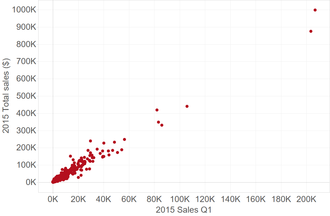
- 2015 Q1 sales is highly correlated with 2015 total sales … Q1 may be a good predictor, especially since we have 2016 Q1 data as well in the dataset.
Distribution of Total 2015 sales; skewed positive. Some outliers, but we first want to check how the model performs without removing outliers

Total 2015 sales vs Total 2015 Q1 sales (all in dollars)
Total 2015 sales vs Average margin per transaction (all in dollars)

(5) Model building
I built a linear regression model with cross validation using scikit-learn, with only 2015 Q1 sales as a predictor of 2015 overall sales. The data was first split into training (70%) and test (30%) data sets, and then a model was fit using the training set. The performance of the model on new data was tested using a 6 fold cross-validation on the training set. Here’s a code snippet and some results.
# Cross-validation
scores = cross_val_score(lm1, Xs_train, ys_train, cv = 6)
predcv = cross_val_predict(lm1, Xs_train, ys_train, cv = 6)
print(scores)
R2_model = metrics.r2_score(ys_train, pred_model)
R2_cv_scores = np.mean(scores)
rmse_model = (metrics.mean_squared_error(ys_train, pred_model))**0.5
rmse_cv = (metrics.mean_squared_error(ys_train, predcv))**0.5

print("R2_model_train: {}, R2_cv: {}".format(R2_model, R2_cv_scores))
print("rmse_model_train: {}, rmse_cv: {}".format(rmse_model, rmse_cv))
Cross-val scores: [0.925 0.974 0.850 0.961 0.929 0.972]
R2_model_train: 0.962, R2_cv: 0.935
rmse_model_train: 9429.3, rmse_cv: 9635.3
This simple model performed quite well on the training data, and was predicted to perform well on new data as well (R2_cv = 0.935, only marginally less than R2_train of 0.962). Let’s see how the model performs on the test set.
R2_test: 0.973, RMSE_test: 10889.1

The model explains 97.3% of the variability in the test set, even with the outliers retained. The model does not need any additional complexity, and it doesn’t seem to be overfitting the data either. So let’s use this to predict sales in 2016.
(6) 2016 projections and conclusions
Using the model generated above, I used 2016 Q1 sales to predict 2016 total sales.
Here are some results from the projections.
- Overall sales are projected to go DOWN by 4.8% in 2016 ($25.74 million) compared to 2015 ($27.04 million)
- Wayne county is projected to have the biggest increase (+558%)
- Delaware county is projected to have the largest decrease (-64%)
Discussion
Depending on what motivated the tax committee to study this topic, the state legislature may view this either as a negative sign (“sales are down, may need to lower rates just enough to increase sales and make up for lost revenues”) or a good sign (“this may have a positive impact on health and social outcomes, we should consider taxing liquor more”). It may be interesting to explore which locations within the counties show big changes in 2016 Q1 sales, and whether particular categories of items are responsible for these changes. It may also be interesting to explore whether weather patterns or sociological/political changes correlate with the largest increases and decreases in certain counties.